EEB 122: Principles of Evolution, Ecology and Behavior

Lecture?26. Population Growth: Density Effects

https://oyc.yale.edu/ecology-and-evolutionary-biology/eeb-122/lecture-26

Population growth is one of those things in ecology that is good to get kind of an intuitive feeling about. And the main thing that you need to grasp about population growth is that it is multiplicative.?What we'll do today is start by talking about density independent growth, and that is basically compound interest,?yielding?exponential growth.?Small differences in interest rates make big differences in outcomes.?The?interest rate on a population is the difference between the birth and the death rate.?

So I want to take you just through the math of doubling time, and you also need to start getting familiar with this kind of notation, because in population dynamics and ecology it is used pervasively.?

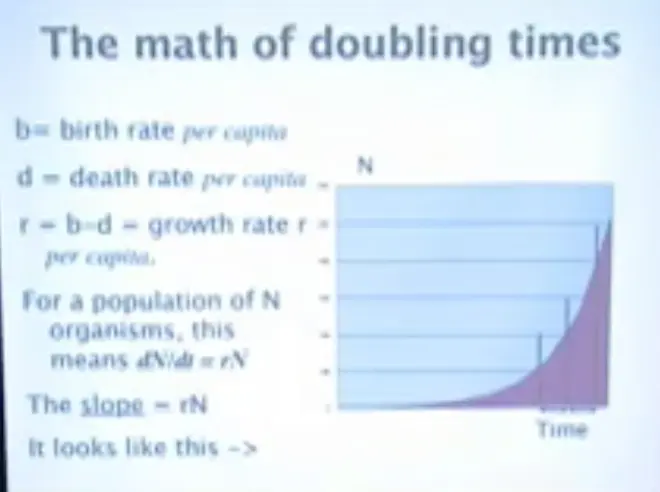
• B?is often used for the birthrate, D?for the death rate, and the per capita growth rate is the birthrate minus the death rate. That's birthrate per capita, death rate per capita, and this is growth rate per capita.

• If you've got?N organisms, then you have the simplest differential equation you can write down practically, which is that the rate of change of the population is equal to the growth rate, times the number of organisms that are present.?

• The slope of population growth is RN. So if we have N on the y-axis, and time on the x-axis, and I put this in to indicate that for a given change in time unit, the amount of growth you get in the population just keeps on going up and up and up.?So the rate of increase in an exponential process is proportional to the growth rate times the amount of stuff that's there; and that's the slope of the relationship.?
  

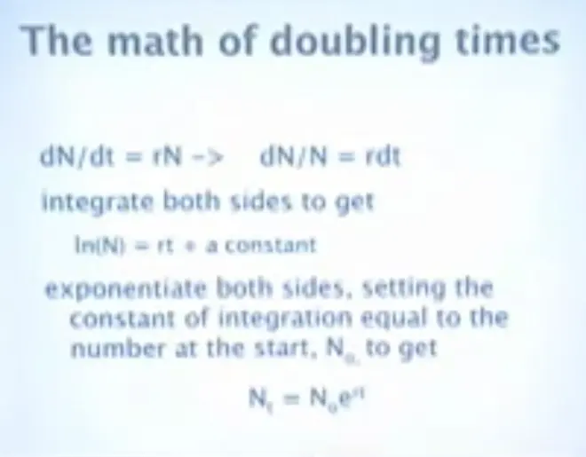
• Then?you get that the natural log of the number of organisms in the population is equal to the growth rate times the amount of time that's elapsed since they started growing, plus some constant. So if you raise E to the log, you get N.

• So the number of organisms you have T-time units later, is equal to the number that you started with, times E, the base of the natural logarithms, raised to R times T. And, in fact, that's the basic compound interest formula as well.

• How long does it take for that population to double? You can divide 69 by the interest rate to get the doubling time.

Now in summarizing this, there was no age structure. All of those numbers that we were counting up represented the population as though every single organism in it had the same probability of reproducing or dying; and that's not true.?

• One of the most obvious things about populations is that organisms of different ages reproduce at different rates and have different risks of dying. So it would be nice to be able to do population dynamics, with a bit more realism, by sticking in all the difference that age structure makes; in other words, doing demography.

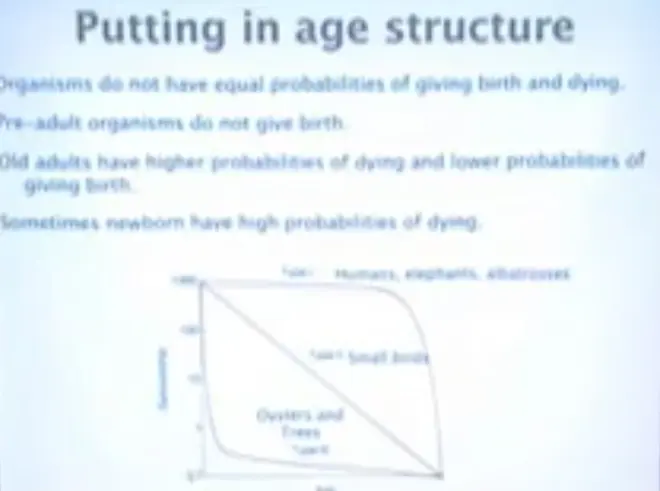
• Pre-adult organisms don't give birth. Old organisms have high probabilities of dying. Newborn have very high probabilities of dying. And if we look around the world, we can see that there are roughly speaking three different kinds of survivorship curves. We have age on the x-axis here,?and?survivorship on the y-axis, in a logarithmic scale.

• The kinds of things that have type-1 survival curves are humans, elephants and albatrosses. Small birds have type-2 survival curves, as do hydra. And oysters and trees have type-3 survival curves; and orchids. They make hundreds of millions, or billions of seeds; most of the seeds die; and once you have made it to adulthood, then your prospects are pretty good.?

We need a bit of demographic notation. There are some of?the key things where people can stumble when they first encounter this notation, and points that you want to make sure you keep in your memory as important distinctions.?

• The first one is the distinction between age and time, and that is the distinction between being 62-years-old and 21-years-old in 2009, and what's happened over the last 20 years. So you can have people of different ages at the same time, and you can have people of the same age at different times. So X keeps track of age and T keeps track of time.

• Then there are two different kinds of ways of thinking about survival. One is the probability of surviving from now to next year, or now to the next time unit, however you choose to scale your time unit.

• And the other is the probability of surviving from birth until now, which would be the probability here, LX, probability of surviving from birth to beginning of age class X.

• Then once you get to be X years old, MX is the symbol that keeps track of how many babies a female would have, that survived to that age. Alpha is age at maturity; Omega is age at last reproduction. And age at maturity doesn't mean, in demography, age at acquisition of secondary sexual characteristics or acquisition of the ability to reproduce, it means the actual age at which a baby arrive or when offspring are born.

• Little-r is the population growth rate. And here we have a collection of three different growth rates, and they mean somewhat different things.?

• r, as I mentioned before, is B minus D, birthrate minus death rate, and it's an instantaneous per capita population growth rate.

• Big Ro is the lifetime expectation of female offspring. In demography we tend to keep track only of females, because they are the rate-limiting sex as their?reproductive rate?actually determines the rate at which the population will grow. So this is the rate of growth per generation, and it's Ro; and Lambda, which is er?is the multiplicative rate of growth per time unit.?

These things are calculated on the basis of life tables. So a life table is an accounting tool, and frankly life tables are a bit like natural selection in the following way; they actually do imply a kind of natural selection, but that's not the point I want to emphasize.?

• LX is the probability of surviving from birth to age X. BX or MX is the number of female offspring?born to females of age X. And LXMX is the probability both of surviving to X and of having MX offspring.

• So the sum, LXMX, over all ages X, is the expected number of female offspring per female per lifetime; that's R0. So you can just put an equals sign in here, that's R0.?So that's a measure of population growth, an important one.?

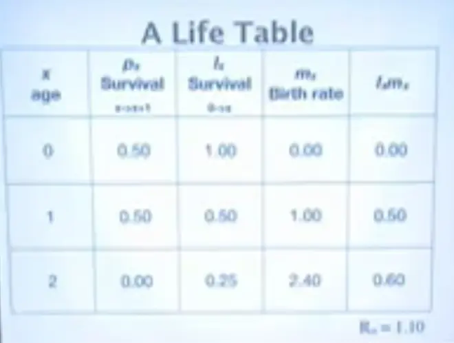
• And if we take a simple example where we have this survival rate from one year to the next--and I've set this equal to 0, so that nobody makes it to age 3--starting at birth everybody--we're keeping track of things that get born--so everybody has a probability of 1 of being born--because those are the only ones we're counting--and 50% of making it to age 1, and 25% of making it to age 2.?P0 times P1 gives us .25.

• So these organisms mature at age 1 and they get better at reproducing; perhaps they continue to grow and they have 2.4 offspring per female at age 2. And these are their contributions to fitness: .5 here; so half of them make it to age 1 and have 1 offspring, and a quarter of them make it to age 2 and have 2.4 offspring. We multiply those numbers together, sum them up, we get R0 = 1.10. The important thing about R0 is that it's greater than 1. This population is growing.?

Now if we want to look ahead and ask what's going to be the age distribution in future years? If you have a life table for humans--you might be interested in knowing will there be enough people around, who are young, to pay for your Social Security when you're old?--you can use this procedure to do so, and that's what demographers do with it.?

• So the number of newborn is the sum across age classes; so the number of females alive that year, times their expected fecundity.?Just take the number of females, take the average number of babies they'll have, and that's the number of newborn.

• The number alive in any older age class is the number that were alive in the younger age class in the previous year, times the probability they survived.?

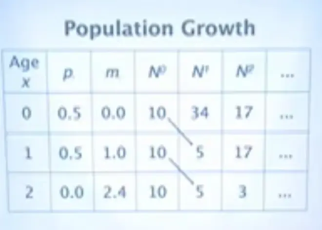
• Now I've put in 10 organisms in each of the three age classes. We have 10 newborn, 10 1-year-olds, and 10 2-year-olds. And this is how the population will develop. Half of these survive, half of these survive. Half of these survive, half of these survive. I've rounded these off to get whole organisms. So that's the survival part of it.

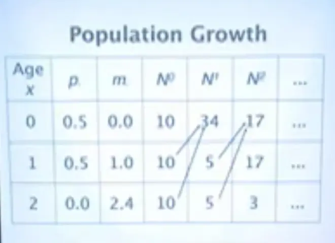
• How about the births? Well these 10 here are going to be giving birth to 5 offspring, and these 10 here are going to be giving, each of these are going to be giving birth to 1 offspring. So that's 10. And these 10 here give birth to 2.4.?Five offspring come from this group and 12 offspring come from this group, and we get 17.?
  

And that just keeps going. So in each generation you can carry that out as a matrix transformation. It's called the Leslie matrix. You can use all of the properties of linear algebra to project things into the future.?

• Any such process, where you have a constant rate of birth and death, will produce a population that attains a stable age distribution in which the proportion of individuals in each class remains constant. So that means like the ratio of five-year-olds to ten-year-olds remains constant. And it will get there not immediately but fairly quickly.

• When it gets into stable age distribution, both the entire population and each age class in it are growing exponentially at the constant rate, r, and that r has exactly the same meaning as it did when we were back dealing with a simple population in just that simple differential equation. The growth rate of the age-structured population is the same as the growth rate of a density independent population.?

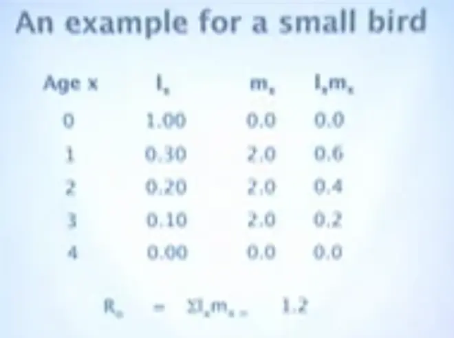
Here's a life table that actually is roughly that of a small bird. So the guys that fly into my bird feeder in Hamden, the house sparrows, the chickadees and so forth, they could have a life table that looks something like this. They don't live very long.?

• So here are the probabilities of surviving to age 1, 2 and 3. Here are the birthrates. I've set them constant for the three age classes. Here's LXMX. This is our population growth rate. It's 1.2 per generation.

• So just based on this, we can make several interesting statements. Their population is growing. And that's because 1.2 is greater than 1.0. And it is multiplying actually 1.2 times per generation; not per year, but per generation.

• We can calculate the generation time with this formula. So we just divide sum of LXMX times X, by R0. That turns out to be 1.67 years. And the meaning in words of generation time, in demography--it's a technical meaning--is the average age of the mother of a newborn. So that's the average age of the mother of a newborn.

• The little-r, can be estimate?by taking the log of big-R and dividing it by the generation time; and that's about 0.11. So this population is growing at a compound interest rate of about 11% per year, and we can use that to go back and use our doubling time calculations to figure out, oh, it's doubling about every 6.3 years. If I'm putting the bird seed out there in Hamden, I had better be ready for large expenditures.

• And I'd like you to note that R0 is calculated on a different time period, generation time, than little-r. So when big-R0 is equal to 1, little-r is equal to 0, and the population is then?stationary; it's just replacing itself. A stationary population is replacing itself, but a population with age structure, that is growing, can be in stable age distribution. Stable age distribution refers to the ratios between the age classes; stationary refers to whether or not it's just replacing itself, or whether it's growing or declining.?

So that's a rough sketch of simple demography, and an introduction to the different ways that ecologists and demographers conceptualize growth rates. Now I want to criticize--not really criticize, but comment on one of the basic assumptions of this.?

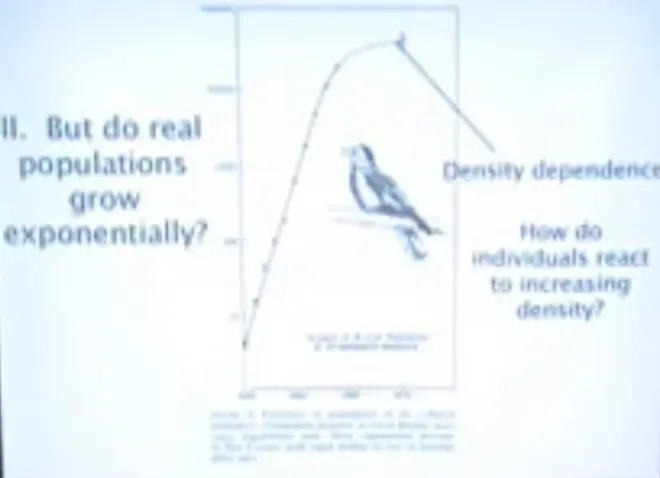
• The first way that you can?complicate?simple dynamics is by putting in age structure, but the second way you can complicate it is by putting in?density. Here is growth of a bird that was introduced to Great Britain,?the turtledove, and it took off from a very small population, and it grew exponentially. If you have a straight line on a semi-log plot--so y-axis here; numbers is on?a log?scale; x-axis is on an arithmetic scale. So this is a straight line, and it's going like gangbusters, it's growing exponentially.

• It's increasing in size about ten times every three years. So these doves are really pumping out the babies and they're surviving pretty well. But something happens up here. This is a real point here; this is a real point here, and it starts to level off.

• So the question is, what does increasing population density do to the demography, the birth probabilities, and the death probabilities of individuals? Can we understand that in terms of the kinds of concepts we're already covered this morning??

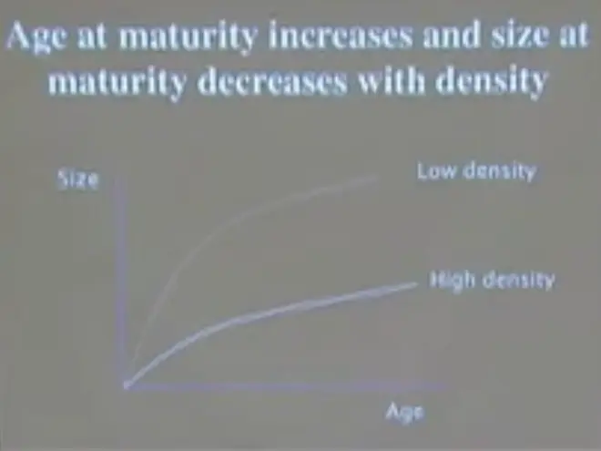
• So as density--we can think of this being a high density population and this being a low density population, with rapid growth, rapid individual growth--now not population growth, but rapid individual growth, increase of size with age at low density, and slow individual growth at high density.

• And I think by now you're familiar with the idea that there is a reaction norm for age and size at maturity. And if you move from low density to high density, basically what happens, is you get organisms that mature later?at a smaller size. So one of the very basic characteristics that determines population growth is age at maturity.

• That's basically the interval over which the compound interest is being calculated, and that's responding plastically to density. So as the density of the population goes up, the organisms delay maturity, they mature later?and they mature smaller.?So they are less capable of making babies, and they're doing so later in life and at a slower rate.?

The other dramatic thing that happens with density is that mortality increases. This is a log scale here and a log scale here, and the flat line here basically indicates that growth has stopped, or that density has stopped increasing.?

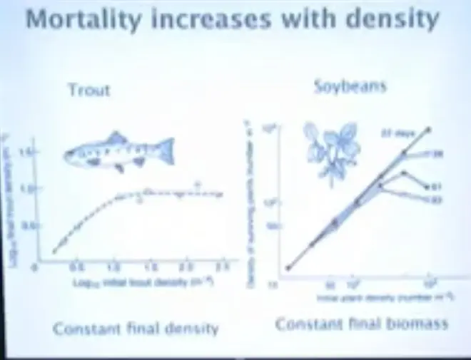
• If you just take an experimental stream bed, and you seed it with baby trout, and you do that a number of times, at different initial densities per square meter.?So this would be 10 raised to the 2.5 per square meter. So this is about 300 trout per square meter, and this is 10 trout per square meter over here. So in arithmetic terms, we're going from 10 per square meter, up to about 300, and what we get out, at the end of the experiment, is roughly 10 per square meter.

• There's an enormous amount of mortality which is going on, over on this end. You can think of that as sort of runt of the litter kinds of things, baby pigs competing in a litter, or you can think of it simply as interspecific competition. These trout are competing for food, and the ones that are best at finding it are going to be the ones that survive.

There've been lots of experiments done with plants. Here again we have a log scale on this axis and a log scale on this axis, and this is the density of surviving plants here.?So this is the number per square meter.

• On this axis we have the number that were planted, and that's going to range from--down here we're probably at about 12 or 15, up to about 1000 per square meter, were planted. And these different lines here are showing you what the density of plants is 22 days after planting, 39 days after planting, 61 days after planting, and 93 days after planting.

• And this is the demographic process that basically leads to constant final biomass. So if you go on, all the way through to harvest, you're going to end up with about 100 plants per square meter, and the--by the way, the way that plants regulate their individual growth, you essentially get the same amount of leaf area or root area covering a square centimeter of ground.

• So if you plant a lot, you're going to end up with fewer leaves and less roots, and you're going to get smaller plants, but the total amount of plant material sitting on that square meter will be roughly constant?irrespective of initial planting density, if you just let this process go on long enough.

The other thing that happens is that as density goes up, fecundity goes down, and that's because as density goes up, competition for food increases, individuals are not getting fed as much, and they are therefore less able to make babies.?

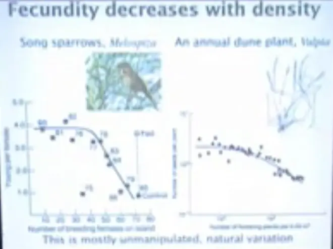
• In this panel over here, we see basically natural variation in song sparrows on Mandarte Island, which is a small island off the coast of Vancouver Island; it's not too far from Victoria. If you take the ferry from Vancouver, over to Victoria, you go within about a kilometer of Mandarte Island.

• And this is the number of young that females were able to fledge. These are the years. So that's 1980, 1981, 1982. This is the number of breeding females on the island. And what you see is that as the number of breeding females increases, the number they are able to fledge starts to decrease.

• And in the year 1985 they did an experiment where they added food--so they wanted to see whether this natural variation could be manipulated, just by putting food out on the island--and those who were fed were able to rear nearly four offspring; and at high density, up here, in 1985, those who were not fed were only able to rear one.

• So there was a difference per female of nearly three offspring, and that was what the population density was doing to them, and the manipulation experiment showed that it was the density and that food was the mechanism.

• If you look at a dune plant in the Netherlands--this is?Vulpia, which is a grass, and this is growing near Leiden, on the dunes on the North Sea in the Netherlands. The number of seeds per plant, number of flowing plants per quarter square meter; the number goes down. So the more crowded they get, the fewer seeds they can make.

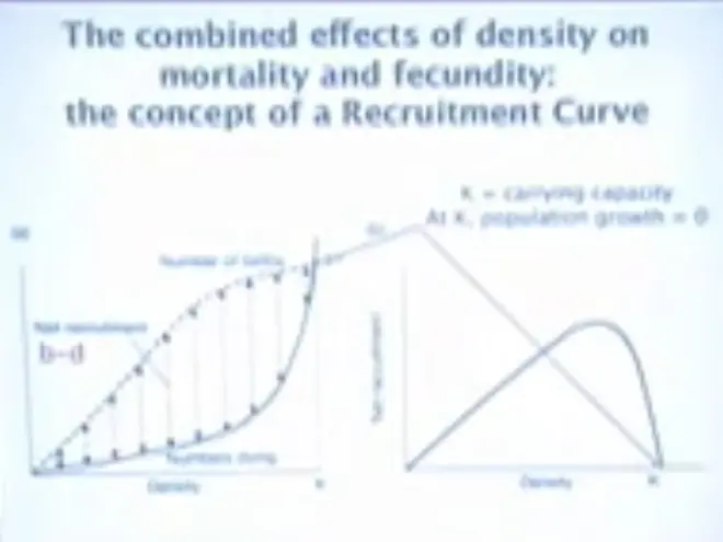
• These effects can be combined. So if we want to combine number of births and numbers dying, this would be density, over here, going from 0 up to a number K.?The numbers dying increase as we go across this, and the numbers being born decrease, and at some intermediate point you have the greatest difference between the births and the deaths, and that difference between births and deaths is the recruitment.

• The recruitment inferred from this graph looks like this, and at 0--you get zero recruitment when you hit this number K; and that number K is called carrying capacity. So the population, under density-dependent regulation, will increase until it hits carrying capacity, and then it will stop growing.?
  

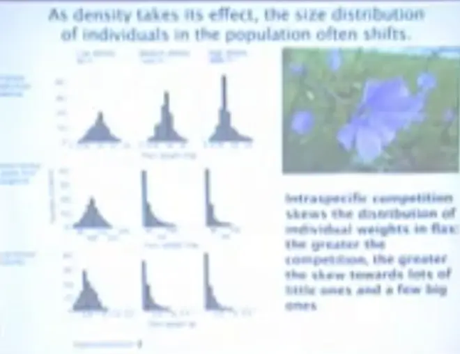
Now as density is taking its effect, the size distribution of individuals in the population often shifts.?

• If you start at low, medium or high density, two weeks after emergence the distribution of body sizes in the population is pretty similar; it's a nice bell-shaped curve. This is now six weeks from emergence. So a bunch of other replicates have now been gathered.

• And you can look at plant weight here, you can see that they're bigger, the scales are changing. But you'll notice that at the medium and at the high-density treatments you're starting to get quite a bit of skew. You're starting to get a few big ones and lots of little ones; that's what this kind of histogram means here, lots of little ones and a few big ones.

• And at the final harvest, which is probably about 12 weeks after planting, you're starting to get a little bit of skew at the low density treatment, but at the medium and high density treatments, you've got a lot of skew.?

Now this is something that was going on?in those trout experiments; you were getting a few big ones and a lot of little ones. In the plants living in the Dutch dunes, you were getting a few big ones and a lot of little ones. It's a pretty widespread pattern that happens as density increases.?

There's going to be intra-specific competition. Some individuals are going to be better at it than others. It's going to result in these kinds of size and growth distributions. So the more competition there is, the greater the skew will be between lots of little ones and a few big ones.?

• That means that competition is producing an asymmetry, and this asymmetry, where you have a really skewed size distribution, just basically means that a few individuals are going to be doing most of the surviving and reproducing, and a lot of individuals are going to be doing most of the dying, and not reproducing.

• In many cases the number of large individuals is relatively constant, while the number of small individuals varies much more widely. That's the law of constant final yield. Or the flat line that we saw with the trout that were seeded into the streams, at many different densities, but you always ended up with roughly the same number. That was probably the number of the large surviving competitive individuals, and the small individuals are being squeezed out.

That has an evolutionary consequence. This is a direct tie now between population dynamics and natural selection.?

• Not all those who are born will survive to reproduce; some are starving or are being crowded out. And not all who survive to reproduce are large and in good shape. Many of them, in fact, are in poor condition and have few offspring.

• Intra-specific competition produces great variation in capacity to reproduce and in reproductive success, and that means that wherever you have reproductive and mortality skew, that's being produced by intra-specific competition, you are generating the conditions for natural selection.?

Populations are held in check by lots of things. They're not just held in check by food. They are held in check by breeding sites, by space, by lots of limiting resources.?

• As populations increase in density, the individuals shift along reaction norms. They reduce growth, they are smaller; when they become adults they experience more variation in adult size; they have lower fecundity and more variation in fecundity; and they have higher mortality and more variation in mortality, as they encounter density dependence.

• If you are?a dominant species in its local habitat, in its ecosystem, then intra-specific competition?is often a more important brake on its growth than inter-specific competition. And that's?because it's dominant, it's numerically abundant, and the average interaction that an individual has is with another individual of the same species, rather than with some individual from another species.

• So that would be a circumstance under which we could expect that intra-specific competition, generating all of these effects, is likely to be important. If the species are rare, or if they're often at a low population density, then the opposite might be the case; then the interactions with other species may be generating these kinds of effects.

• But whether the effects are generated by interactions with other individuals of your own species, or individuals of another species, the impact of increased overall density is likely to be qualitatively similar. It's going to produce reduced growth, smaller adult size, lower fecundity, higher mortality, and more variation in all of these parameters.?